Decision Trees in Machine Learning
Machine Learning is one of the most attractive career options available to us today. While the demand for Machine Learning engineers and the salary packages offered are definitely good motivations, another factor which attracts people is the way in which it mimics the human decision making and solves our problems.
Decision trees in Machine Learning are some of the simplest and most versatile structures which are used extensively for classification purposes. A decision tree in Machine Learning is fundamentally a “tree” of decisions that make up the nodes where "branches" are split from the tree. Take a look at the diagram below for an example of a decision tree.

Each node and sub-node is a decision based on the value of certain variables which ends with the classification of each element into one of the classes. The first variable which divides the data set is known as the root. It’s where everything starts from. Every other decision is called a node and every line connecting the decisions is a branch.
Decision trees in Machine Learning can be easily visualized through the tree structure shown above.
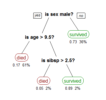
A Decision Tree in Machine Learning has been used in order to classify passengers who survived the sinking of the Titanic. At each node in the decision tree is a decision that helps predict whether or not the passenger will survive the Titanic disaster. Here, “sibsp” is the number of spouses or siblings aboard the ship. The final node determines the classification of the passenger on whether they survived or not.
This type of tree is called a classification tree as it is used to solve classification problems.
Decision Trees in Machine Learning – Splitting Candidates
Decision trees in Machine Learning are made by taking data from the root node and splitting the data into parts. If we look at the Titanic example, the splitting of the data is determined by our intuition of what makes the most sense and is confirmed from the data that we have taken the right decision. One of the most important decisions that we have to take in regards to Decision trees is the best way in which the data has to be split. This can be done on the basis of instinct or through an algorithm. Decision Trees in Machine Learning generally have their splits based on the dataset given.
The Numerical features can be split according to the data we see. There can be several different methods through which the data can be split. One of the more common ways to split the data based on threshold values. These threshold values are determined after sorting the data and deciding on the best way to split the data based on this. We can also cut them straight down the middle. There are too many splitting algorithms to discuss here so we might as well go for a simple algorithm.
(1, a), (2, b), (1, c), (0, b), (3, b)
In the rudimentary data given above, we can see three classes (a, b, c). The first thing we do is put them into different categories.
{(0, b)}, {(1, a), (1, c)}, {(2, b)}, {(3, b)}
Now we have 4 different sets. There are several resources available on the internet to learn about set theory.
As an example, the sets can be splits arbitrarily:
Split 1 <= 0.5
Split 2 <= 1.5 but > 0.5
Split 3 > 1.5
This is one of the ways in which the decision trees can be split. It is important to have an idea of the data before the splitting is decided.
How to find the best Splits for Decision Trees in Machine Learning
One of the hardest things about determining the split in the Decision Trees in Machine Learning is trying to find the smallest decision tree which has a reasonably high classification accuracy.
So, in place of getting the best result, the best thing that can be done is to find the solution which is closest to the best result which will be easier and faster.
The objective of the decision tree is to explicitly split the data into the number of divisions required. The decision tree should be able to divide the data into the classes without impurity. Each class should be clearly divided in the decision tree.
This measure of purity is called information. It represents the expected amount of information that would be needed to specify whether a new instance should be classified as the left or right split.
To find the best splits, we need to learn a few things first.
Expected Value
The expected value is simply the estimated value of the experiment that is run. You can use this to work out the average score of a dice roll over 6 rolls, or anything relating to probability where it has a value property.
Suppose we’re counting types of bikes, and we have 4 bikes. We assign a code to each bike like:
001, 010,011, 100
For every bike, we give it a number. For every coding, we can see we use 2 bits- either 0 or 1. In order to find the expected value, the probability of each bike being chosen has to be calculated. Each bike, in this situation, has equal probability. So each bike has a 25% chance of appearing.
Calculating the expected value we multiply the probability by 2 bits, which gets us: 2
Advantages of Decision Trees in Machine Learning
The use of decision trees in Machine Learning is quite extensive. Some of the biggest advantages, which make it widely used, are:
- Simple to understand, interpret and visualize.
- Decision trees implicitly perform variable screening or feature selection.
- Can handle both numerical and categorical data. Can also handle multi-output problems.
- Decision trees require relatively little effort from users for data preparation.
- Nonlinear relationships between parameters do not affect tree performance.
Disadvantages of Decision Trees in Machine Learning
While there are extensive uses of Decision Trees in Machine Learning, this does not mean that there are no disadvantages to the technique. Some of the more prominent disadvantages are:
- Decision-tree learners can create over-complex trees that do not generalize the data well. This is called overfitting.
- Decision trees can be unstable because small variations in the data might result in a completely different tree being generated. This is called variance, which needs to be lowered by methods like bagging and boosting.
- Greedy algorithms cannot guarantee to return the globally optimal decision tree. This can be mitigated by training multiple trees, where the features and samples are randomly sampled with replacement.
- Decision tree learners create biased trees if some classes dominate. It is therefore recommended to balance the data set prior to fitting with the decision tree.